Excel Re-Imagined

There are many sophisticated reporting and budgeting, forecasting and analysis tools on the market. Much of the marketing messaging around that software challenges us to ditch Excel in favor of their tool. They tell us Excel workbooks are prone to errors, don’t scale well, don’t handle succession well, and are subject to file corruption. It may all be true. But when everybody else has left for the day, we head back to our office and check those numbers in Excel.

In September 2018, Microsoft released seven new Excel functions to Office users subscribed to the Microsoft Insiders program. These are now generally available to Excel users. The new functions: UNIQUE, SORT, SORTBY, FILTER, RANDARRAY, SEQUENCE and SINGLE, can return multiple values, or dynamic arrays, to their own and neighboring cells. The result is a completely new set of Excel-based tools in the hands of business officers. In this new series of article we’ll look at these functions and how they trigger a whole new way of working inside Excel.

But first, we need to understand some changes to the Excel calculation engine.

Dynamic Arrays

Arrays: A set of elements that have some property in common.

In Excel, much of what we do involves working with an array. We are either processing the array in some way or analyzing it to discover useful information. Arrays can be either used as the output, or as a source for a lookup. Example: An array might be a list of US states or Canadian provinces with columns for their 2-letter identifier and their name. That array is pretty much static – there is no immediate expectation that it will add or lose members.

In Excel, a dynamic array is an array that can change. If the result of one of the new Excel functions returns a dynamic array that might not be limited to a single cell, that has to change the design of many spreadsheets.

To see if the version of Excel you are running supporting dynamic arrays, try this simple test.

Type a sequence of numbers in cells A1 through A4.

In cell B1, type ‘=A1:A4’ and press <Enter>

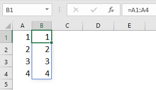
If your version of Excel supports dynamic arrays, the result of the short formula you typed in B1 will spill from from B1 to B4.

Spilling

Where we previously used array formulas (where we would press <Ctrl><Shift><Enter>), now it is sufficient to type in a formula and provide room on the sheet for the result to spill.

Or, if we previously typed one formula, then filled it down, we can now type a single formula, and the updated Excel calculation engine will spill the results. This works for the new Excel functions we’ll discuss in subsequent articles, but also previously existing functions.

In the example at the right, the ROUND() function spills when provided with a range as the first argument.

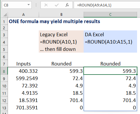
This behavior is exhibited both vertically and horizontally – a result spills down, or to the right.

Note the blue border around the results is a visual cue to the fact that the values in those cells are spilled formula results.

To delete spilled data, delete only the formula at the top of the column.

Cell formatting does not spill. However, formatting can be applied to the cells into which results spill.

In formulas that rely on the spilled data, a good way to reference the spilled result is to use the # sign. In the illustration of the ROUND() formula above, one could type a formula that refers to C8# that will then include the results from C8 to C13.

If there is data that interferes with the range to which data would spill, the formula returns a #SPILL error, and the range that must be cleared is outlined in a dashed blue border.

Over the next few articles, we’ll take a look at some of the new Excel functions that leverage the new capabilities of the redesigned Excel calculation engine.