
Excel UNIQUE Function

This continues a multi-part discussion of some new features introduced in Excel in 2019 and 2020. This describes the capabilities of the UNIQUE function, especially when used in combination with previously reviewed dynamic array functions SORT and FILTER. For a discussion of dynamic arrays, see the intro to this series.
Usage
This is the function for which many have been waiting for some time. UNIQUE returns a list of unique values from a longer list. This functionality can also be provided by using a pivot table, or sorting and grouping a list. But in both of those situations, the resulting list does not update automatically as the dynamic array returned by UNIQUE does.
Arguments
The arguments are as follows.
| UNIQUE(array, [by_col], [exactly_once]) |
|---|
| array = Columns included in the result. Can be entire or part of source data set. |
| by_col = If data is in rows instead of columns, use TRUE. Default is FALSE or 0. |
| exactly_once = TRUE returns values that occur only once in the data set. FALSE returns values that occur once or more. Default is FALSE. |
Examples
These examples are available for download in the demo workbook. Sample data is fictional but is set in the context of a post-secondary institution.
Example 1
Starting with a raw list of financial transactions in a table called AR_Transactions that would be either linked to or exported from an accounting system, the objective is to compute current account balances.
Two formulas can be used to set this up. In F2, use the UNIQUE function to return a list of the names of students with transactions in the list. For readability, use the name of the table and column, rather than referring to the explicit cell range that includes the table and column.
=UNIQUE(AR_Transactions[Student])
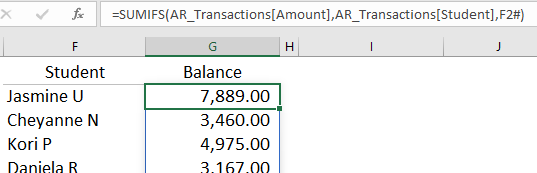
In G2, use SUMIFS to simply add all the of transactions for each student.
=SUMIFS(AR_Transactions[Amount],AR_Transactions[Student],F2#)
The F2# refers to the entire dynamic array returned by UNIQUE into F2 and spilling down.
In the demo workbook for download, the SORT_UNIQUE worksheet has exactly the same data and table, but nests UNIQUE inside the SORT function to return a sorted list of student names.
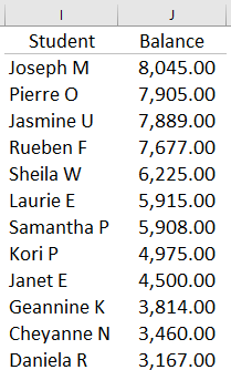
Of course, the most frequent question here is which student owes the most? A simple way to show this is to set up a dynamic array in cell I2 using this formula.
=SORT(F2#:G2#,2,-1)
This returns the spilled results in F2 and G2, sorts by the second column (the Balance), in descending order.
Example 2
In this example, UNIQUE is used in combination with SORT to check for address errors or inconsistencies in a dataset of donor records.
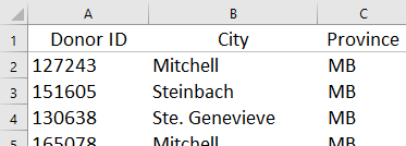
The donor information is in a list in columns A to C. The data in this set is of course completely fictionalized, but the names of towns are from central Canada where Plains Edge is based.
Cells E2 and F2 contain the following formulas.
E2   =SORT(UNIQUE(B2:B301))

F2   =SORT(UNIQUE(C2:C301))
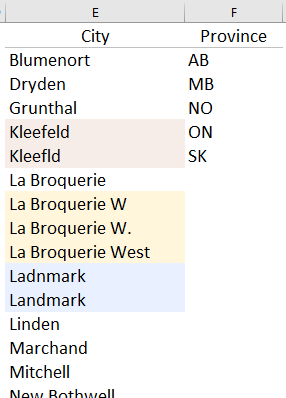
By sorting the unique results, many errors in the addresses are revealed. The village of Kleefeld is spelled two different ways, La Broquerie West is sometimes abbreviated in two different ways, and the name of Landmark is spelled incorrectly at least once.
Canadian provinces, like US states, can be abbreviated with two letters. AB and MB are correct abbreviations for Alberta and Manitoba. However, NO is not a valid identifier and is probably a transposition error for ON, or Ontario.
Application
In practice, the UNIQUE function is a tool that is often useful when evaluating a large dataset. How many customers are represented in the table? How many classifications are actually in use?
Used in combination, UNIQUE, SORT and FILTER functions can be used to create dynamic arrays in a wide variety of situations.
Download the UNIQUE demo workbook.
Here are links to the Microsoft documentation for the UNIQUE function.