A final function to complete the dynamic array toolkit. Like some other DA functions, the function appears simple at first, but provides great versatility when combined with other DA functions such as UNIQUE, SORT and FILTER. For a discussion of dynamic arrays, see the intro to this series.

Usage

SEQUENCE provides the ability to create dynamic sequences of numbers or dates. This function is helpful with setting up amortization tables or forecasting models. It can even be used at the core of a dynamic calendar.

Arguments

The arguments are as follows.

SEQUENCE(rows, [columns], [start], [step])
rows = The number of rows to which the result should spill.
columns = The number of columns to which the result should spill. Default is 1.
start = Start number or date. Default is 1.
step = Amount by which the result should change. Default is 1.

Examples

The examples below are available for download in the SEQUENCE demo workbook.

Example 1

To generate a column of 20 numbers starting at 10 and stepping by 10, the function would be as below.

=SEQUENCE(10,1,10,10)

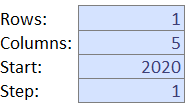
To set up a row of years, starting from 2020 for a 5-year forecasting model, use the following formula.

=SEQUENCE(1,5,2020,1)

Example 2

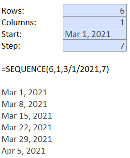
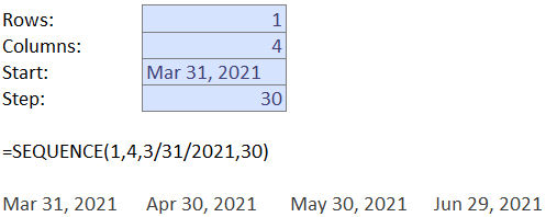
In the SEQ_Dates worksheet the function is similar, but results are formatted as dates.

With this example, one could generate a column of the next 6 Mondays, starting March 1, 2021, or column headings for an Accounts Receivable aging report.

Example 3

Until dynamic arrays were available in Excel, it was most common to provide scalar arguments to functions, that is, arguments that had a single value. However, now many Excel functions will accept arrays as arguments as well. This opens up many possibilities, especially for the SEQUENCE function.

(For those familiar with array or CSE or <Ctrl><Shift><Enter> formulas, that was and still is a way to work with array-based arguments and results. Though that capability is not dynamic in the way that the new DA functions are.)

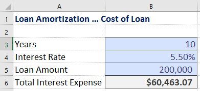
On the LoanCost worksheet of the demo workbook, the objective is to calculate total cost of a loan, provided with loan duration, interest rate and loan amount. This can be calculated in a single cell in B6.

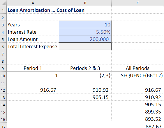
Start by reviewing the formula in cell A12. This uses the IPMT() function to calculate the interest portion of the loan payment for period 1.

=-IPMT(B4/12,1,B3*12,B5)

The second argument in the IMPT() function is the period for which to calculate interest. In cell B12, the 1 (scalar value) has been replaced with an array {2;3}. An array is formatted between curly brackets and separated by a semi-colon. This causes the result to spill, and return the interest portion of the loan payments for periods 2 and 3.

=-IPMT(B4/12,{2;3},B3*12,B5)

The formula in cell C12 then takes this to the next level by replacing the array {2;3} with a SEQUENCE() function containing all the values for the months in the loan, or B3 (loan duration in years) X 12.

=-IPMT(B4/12,SEQUENCE(B3*12),B3*12,B5)

Finally, to calculate total interest cost of the loan defined in cells B3 to B5, enclose the formula in cell C12 in a SUM().

=SUM(-IPMT(B4/12,SEQUENCE(B3*12),B3*12,B5))

Example 4

In the LoanAm worksheet, the SEQUENCE() function plays a key role in the construction of a dynamic loan amortization table.

Cells B3 to B5 contain the same inputs as the previous example. Cell B6 now uses the Excel PMT() function to calculate the monthly loan payment.

Cell D10 starts the amortization table with the initial loan amount.

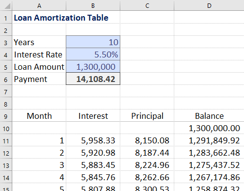
In row 11, the table calculations begin.

The Month column uses SEQUENCE() to return the month numbers, based on loan duration in years multiplied by 12.

The Interest column uses IPMT() function together with SEQUENCE to calculate monthly interest, as demonstrated in the previous example.

The Principal column subtracts the interest from the payment. To use the correct amount of interest for the month, the formula references B11#, or the array of values calculated in the Interest column.

Finally, the running Balance column uses a nested SUMIFS() function to reduce the loan balance by the total principal paid to date.

Next…

Bonus: The SEQUENCE demo workbook contains a Calendar worksheet which demonstrates a dynamic month calendar based on the use of SEQUENCE(), WEEKDAY() and IF().

While this wraps up the series of posts about functions released to specifically leverage the dynamic array capabilities in Excel, two additional posts will cover the versatile XLOOKUP() function and the new LET() function.

Download the SEQUENCE demo workbook.

Here is a link to the Microsoft documentation for the SEQUENCE function.