

Excel SORT Function
This is part of a multi-part discussion of some of the new features introduced in Excel in 2019 and 2020. This post is about one of the new dynamic array functions. For a discussion of dynamic arrays, see the intro to this series.
Usage
SORT does exactly what its name suggests. However, because it updates automatically, it is often a superior choice than a pivot table.
Arguments
The arguments are as follows.
| SORT(array, [sort_index], [sort_order], [by_col]) |
|---|
| array = Columns included in the result. Can be entire or part of source data set. |
| sort_index = The column index on which to sort. Default is 1. |
| sort_order = 1 for ascending, -1 for descending. Default is 1. |
| by_col = If data is in rows instead of columns, set to TRUE. Default is FALSE. |
Examples
These examples are all in the SORT demo workbook available for download. Note that data in the samples is fictional but is set in the context of a post-secondary institution.
Descending Order Sort
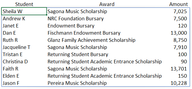
Using the list of student awards in range A2:D120, the following formula returns the set composed of student name, award name and amount (range B2:D120) sorted on the third column (the amount), in descending order.
=SORT(B2:D120,3,-1)
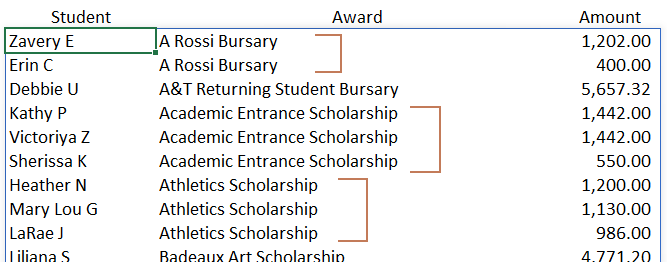
Multi-Column Sort
Using comma-separated arrays as arguments, it is fairly simply to define multiple sort columns and sort orders for each column.
To continue our example with student award data in A2:D120, we use SORT to retrieve 3 columns, the range B2:D120. Column 1 is the student name, column 2 the name of the award, and column 3 is the award amount. When we refer to index, we refer to the number of the column. To sort by column 2, then by column 3, we would put the 2 and then 3 inside curly brackets. {2,3}.
We’d also like to sort the awards in alphabetical ascending order, but continue to sort awards in descending order. For our sort_order argument, we then enclose a 1, then a -1, in curly brackets. {1,-1}.
Putting it all together, our SORT function is as follows:
=SORT(B2:D120,{2,3},{1,-1})
The SORTBY Function
When it is necessary to sort by a column that should not be included in the result, the SORTBY function can be used. The arguments for this function are as described below.
| SORTBY(array, [sort_array], [sort_order]) |
|---|
| array = Columns included in the result. Can be entire or part of source data set. |
| sort_array = The column on which to sort. |
| sort_order = 1 for ascending, -1 for descending. Default is 1. |
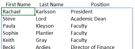
In the following example, staff names, positions and annual salaries are list in a table in A1:D16. This is formatted as a table (<ctrl><T>) named Staff. Using named tables with descriptive column names makes formulas much more readable.
The desired result is a list of names and positions, sorted in descending order by salary, without showing the salary. The SORTBY function identifies the array as Staff[[First Name]:[Position]], selecting the first three columns. The second argument identifies Staff[Salary] as the sort column. The final argument of -1 orders the result set in descending order.
=SORTBY(Staff[[First Name]:[Position]],Staff[Salary],-1)
In the final example, on sheet SORTBY2 of the demo workbook that can be downloaded here, the SORTBY and IF functions are used in a simple auditing tool to identify check numbers issued out of date sequence.
SINGLE
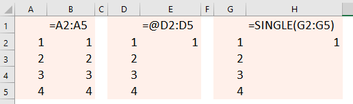
There are situations when the SORT or FILTER functions return an array, but a scalar, or single, result is required. In these situations, the function can be prefaced with the @ sign, or nested inside the SINGLE function.
In the demo workbook on the SINGLE worksheet, the formula in B2 is =A2:A5. The result spills down from B2 to B5, as we have come to expect when working with array functions. However, in cell E2, the formula is =@D1:D5. In this case, the result is limited to a single value in E2. The same thing is accomplished with the =SINGLE(G2:G5) in cell H2.
Given a table named Employees in the range A1:D16, the SINGLE and SORTBY functions can be combined in a formula to return the name of the single highest-paid employee in the table.
=@SORTBY(Employees[Name],Employees[Salary],-1)
Looking Ahead
The SORT and SORTBY functions are deceptively simply. However, as we will begin to see in future posts, combining these with other functions unlocks some of their amazing potential.
Download the SORT demo workbook.
Here are links to the Microsoft documentation for the SORT, the SORTBY and the SINGLE functions.

Excel FILTER Function
This is part of a multi-part discussion of some of the new features introduced in Excel in 2019 and 2020. This post is about one of the new dynamic array functions. For a discussion of dynamic arrays, see the intro to this series.
Usage
FILTER is used to return a subset from a larger set of data based on specific criteria. It can even be used to return non-adjacent columns from the source set.
FILTER is a more flexible alternative to a pivot table, and can handle exceptions in a more robust manner than VLOOKUP.
Arguments
The arguments are as follows.
| FILTER(array, include, [if_empty]) |
|---|
| array = Columns included in the result. Can be entire or part of source data set. |
| include = Test to define what is included in result |
| if_empty = Result to return if filter returns no results. Default is at #CALC! error. |
Examples
These examples are all in the FILTER demo workbook available for download. Note that data in the samples is fictional but is set in the context of a post-secondary institution.
Simple Subset
In this first example, we are looking for a list of students who have received awards greater than $3,000 and the name of the award they received.
The entire list of awards is in the range B2:D120.
We type the following formula in cell F8:
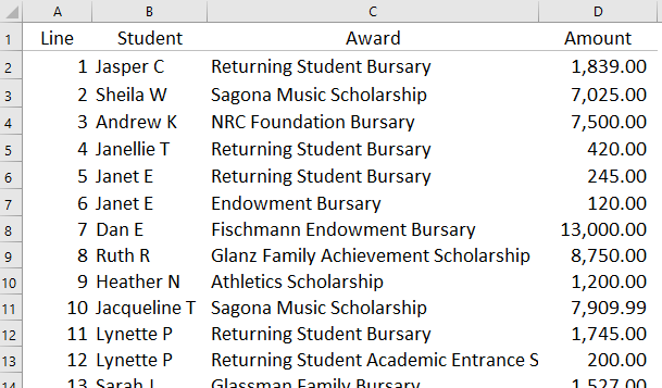
=FILTER(B2:D120,D2:D120>3000,"None")
This returns only the columns we need with the student name, name of award, and amount of award where the amount of the award (in D2:D12) is greater than 3000. In the event that no awards exceed 3000, the formula would simply return the word “None”.

Of course, ‘>3000’ in the formula could be replaced with a reference to a specific cell, such as ‘>$G$5’ which could contain 3000 or any other value on which the return set should be filtered.
Multiple Filter Criteria
It is also possible to filter on more than one criteria. In this example, we would like to see awards with amounts between 3000 and 5000. This can be accomplished by placing the criteria in brackets and multiplying them.
=FILTER(B2:D120,(D2:D120>3000) * (D2:D120<5000),"None")
Multiplying the criteria combines these in a logical AND relationship. Adding the criteria would be the same as setting up OR criteria.
If we are looking for outlier points in our dataset of student awards, perhaps those with awards less than $200 or greater than $7,000, we would add the two criteria.
=FILTER(B2:D120,(D2:D120<200) + (D2:D120>7000),"None")
The result below then show only the small and the large awards, based on the criteria we specified.
Return Non-Adjacent Columns
By nesting one FILTER formula inside another, it is possible to return non-adjacent columns. In this final example, we would like to know which students received awards greater than $7,000, but we are not concerned with the type of award. Since the student name and award amount are not in adjacent columns, this poses a challenge since we can not specify multiple ranges in the first FILTER argument.
However, we can achieve our objective by nesting one FILTER formula inside another.
First we use FILTER to return columns B to D, filtering on the amount in column D.
Then we filter that result to return only the first and third columns, using an array of 1’s and 0’s to indicate which columns should be returned.
Note also that we have replace the third argument inside the inside FILTER function with an array of 3 values, {“None”,0,0}. Should there be no results greater than $7,000, our inside FILTER will return a result array with a width of 3 columns, suitable for the outside FILTER function to parse. Otherwise the outside FILTER function would return a #VALUE! error.
=FILTER(FILTER(B2:D120,D2:D120>7000,{"None",0,0}),{1,0,1})
Looking Ahead
This wraps up our quick introduction to the FILTER function. In future posts we’ll discover how combining FILTER with other new functions such as SORT and UNIQUE opens up intriguing new possibilities in Excel.
Download the FILTER demo workbook.
Here’s a link to the Microsoft documentation for the FILTER function.

Excel Re-Imagined
There are many sophisticated reporting and budgeting, forecasting and analysis tools on the market. Much of the marketing messaging around that software challenges us to ditch Excel in favor of their tool. They tell us Excel workbooks are prone to errors, don’t scale well, don’t handle succession well, and are subject to file corruption. It may all be true. But when everybody else has left for the day, we head back to our office and check those numbers in Excel.
In September 2018, Microsoft released seven new Excel functions to Office users subscribed to the Microsoft Insiders program. These are now generally available to Excel users. The new functions: UNIQUE, SORT, SORTBY, FILTER, RANDARRAY, SEQUENCE and SINGLE, can return multiple values, or dynamic arrays, to their own and neighboring cells. The result is a completely new set of Excel-based tools in the hands of business officers. In this new series of article we’ll look at these functions and how they trigger a whole new way of working inside Excel.
But first, we need to understand some changes to the Excel calculation engine.
Dynamic Arrays
Arrays: A set of elements that have some property in common.
In Excel, much of what we do involves working with an array. We are either processing the array in some way or analyzing it to discover useful information. Arrays can be either used as the output, or as a source for a lookup. Example: An array might be a list of US states or Canadian provinces with columns for their 2-letter identifier and their name. That array is pretty much static – there is no immediate expectation that it will add or lose members.
In Excel, a dynamic array is an array that can change. If the result of one of the new Excel functions returns a dynamic array that might not be limited to a single cell, that has to change the design of many spreadsheets.
To see if the version of Excel you are running supporting dynamic arrays, try this simple test.
Type a sequence of numbers in cells A1 through A4.
In cell B1, type ‘=A1:A4’ and press <Enter>
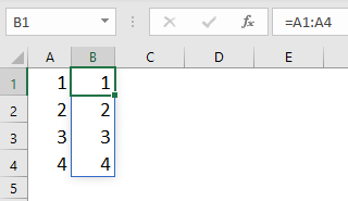
If your version of Excel supports dynamic arrays, the result of the short formula you typed in B1 will spill from from B1 to B4.
Spilling
Where we previously used array formulas (where we would press <Ctrl><Shift><Enter>), now it is sufficient to type in a formula and provide room on the sheet for the result to spill.
Or, if we previously typed one formula, then filled it down, we can now type a single formula, and the updated Excel calculation engine will spill the results. This works for the new Excel functions we’ll discuss in subsequent articles, but also previously existing functions.
In the example at the right, the ROUND() function spills when provided with a range as the first argument.
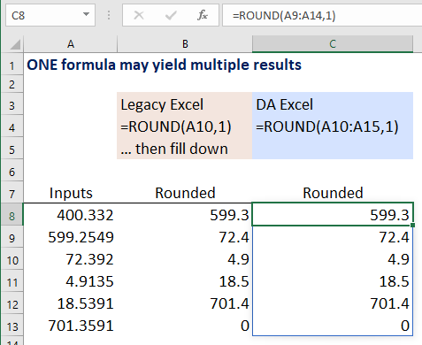
This behavior is exhibited both vertically and horizontally – a result spills down, or to the right.
Note the blue border around the results is a visual cue to the fact that the values in those cells are spilled formula results.
To delete spilled data, delete only the formula at the top of the column.
Cell formatting does not spill. However, formatting can be applied to the cells into which results spill.
In formulas that rely on the spilled data, a good way to reference the spilled result is to use the # sign. In the illustration of the ROUND() formula above, one could type a formula that refers to C8# that will then include the results from C8 to C13.
If there is data that interferes with the range to which data would spill, the formula returns a #SPILL error, and the range that must be cleared is outlined in a dashed blue border.
Over the next few articles, we’ll take a look at some of the new Excel functions that leverage the new capabilities of the redesigned Excel calculation engine.