

Excel LET Function
Photo by Unsplash
Released for Office 365 recently, the new LET function brings clarity and transparency to spreadsheets by assigning names to the results of calculations.
Usage
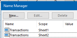
The use of named ranges in Excel is a good way to help other users understand the workbook. When setting up named ranges, Excel makes the name available for use in the entire workbook by default. However, by restricting the scope to a single worksheet, one can use the same name repeatedly in the same workbook.
It is important to be aware of the scope of a name’s availability.
Now with the introduction of LET, it is possible to further restrict the scope of a name to a single cell.
Arguments
| LET(name1, value1, [name2], [value2], … [namen],[valuen], calculation) |
|---|
| name1 = The name of the first value. |
| value1 = Value assigned to the first name. |
| name2, value2 … namen, valuen = Optional additional sets of names with values. |
| calculation = Calculation that uses names defined by previous arguments. |
One can provide multiple name/value sets before using these in the final calculation. These sets can perform calculations using names defined earlier.
Example 1
In the example in the Amort worksheet of the LET demo workbook, the objective is to calculate the annual straight-line amortization cost of some assets, given cost, useful life and salvage value.
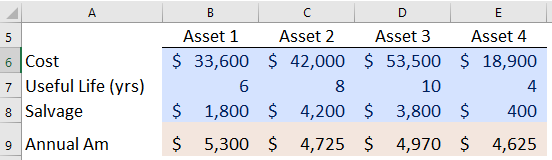
The calculation would be simple enough with =(B6-B8)/B7.
But setting out the calculation in the LET function adds clarity and reduces the chance of a calculation error.
=LET(cost,B6,life,B7,salvage,B8,(cost-salvage)/life)
Example 2
Another common situation arises when working with the IF function. A calculation is performed once to determine whether a condition is met, then carried out a second time for the result.
In the example in the BudgetChange worksheet, operating expense budgets for departments of the University of Manitoba are compared and areas with greater than a 5% budget increase are highlighted.
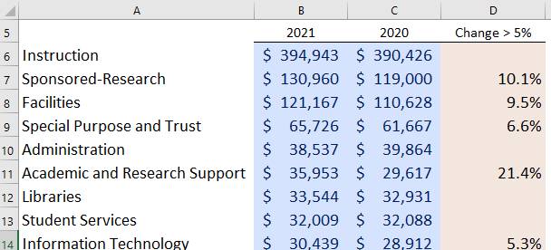
A way to accomplish this is with the formula below.
=IF((B6-C6)/C6>0.05,(B6-C6)/C6,"")
However, LET provides a more readable, albeit longer, formula.
=LET(CurrentBudget,B6,PriorBudget,C6,PercentChange,(CurrentBudget-PriorBudget)/PriorBudget,IF(PercentChange>0.05,PercentChange,""))
To improve readability, add linefeeds after each set of name and value. When entering the formula, press <Alt><Enter> after each set.
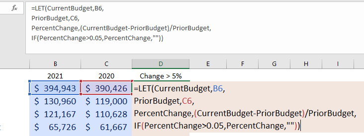
=LET(CurrentBudget,B6,
PriorBudget,C6,
PercentChange,(CurrentBudget-PriorBudget)/PriorBudget,
IF(PercentChange>0.05,PercentChange,""))
In the AverageChange worksheet, the percent change is returned for all departments. The data has now been set up in a table to provide additional clarity, so the formula in the Average Change column uses column names and returns an array.
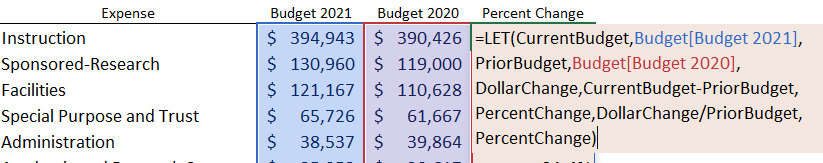
=LET(CurrentBudget,Budget[Budget 2021],
PriorBudget,Budget[Budget 2020],
DollarChange,CurrentBudget-PriorBudget,
PercentChange,DollarChange/PriorBudget,
PercentChange)
At this point, the formula is practically written in English and contains no cell references that are not named.
Recommendation
Any time a longer formula contains more than one instance of the same calculation, consider using the LET function to improve readability and performance of the formula.
Download the LET demo workbook.
Here is the links to the Microsoft documentation for the LET function.

Excel XLOOKUP Function
Photo by Rui Matayoshi on Unsplash
For those using the VLOOKUP or HLOOKUP functions, here is a helpful replacement for both. XLOOKUP brings many improvements to formulas used to find results within a set of data. These include the ability to find values in columns without regard to their relative position to each other, to handle errors more predictably, to search for partial matches and to return multiple results in a dynamic array.
Usage
| XLOOKUP(lookup_value, lookup_array, return_array, [if_not_found], [match_mode], [search_mode]) |
|---|
| lookup_value = The value to look up. Same as with HLOOKUP or VLOOKUP. |
| lookup_array = The array (or column) to search. |
| return_array = The array (or columns) from which to return a result. |
| if_not_found = If no match is found, return this text or value. If no argument supplied, XLOOKUP will return #N/A. |
| match_mode = Start number or date. Default is 1. |
| search_mode = 1 – search in ascending order; 2 – search in descending order. Default is 1. |
Example 1
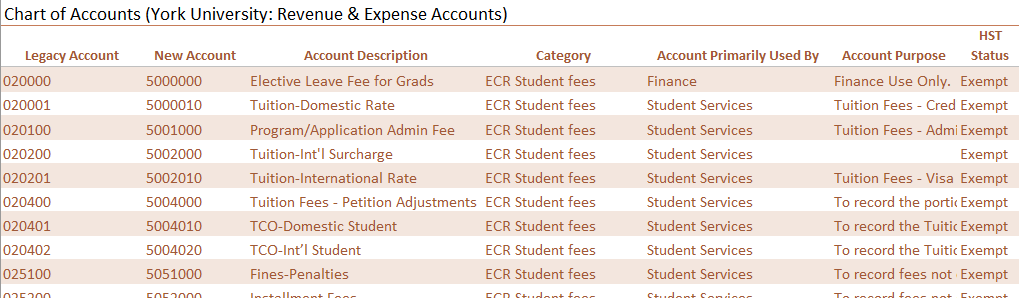
All of the examples below are available to download in the XLOOKUP demo workbook. The examples use revenue and expense accounts from York University. In this fictional scenario, the institution has moved from a six to a new seven-digit account numbering system to make room for additional accounts. For staff to use during and after the transition, a tool is required to lookup account numbers. A table has been set up with legacy and new account numbers for this purpose.
With the legacy account number in column A on the far left, it is simple enough to use VLOOKUP to find the new account number in a column to the right. This is the function in B9.
=VLOOKUP(B8,Accounts1[[Legacy Account]:[New Account]],2,FALSE)
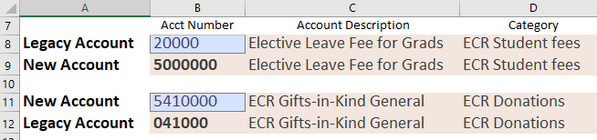
However, it is equally important to be able to look up the legacy account number given the new account number. To do this without XLOOKUP, one might use INDEX and MATCH, or set up a duplicate table of accounts but with columns A and B swapped.
With XLOOKUP neither method is necessary. Rather, one specifies the lookup and return columns, or arrays.
=XLOOKUP(B11,Accounts1[New Account],Accounts1[Legacy Account],"No match",0,1)
Further, the formula provides a predictable response in the event that the lookup value is not found.
Example 2
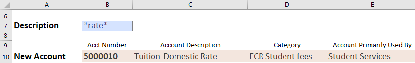
XLOOKUP allows a lookup of a partial match using special characters * and ?.
? represents a single character, while * takes the place of multiple characters.
In the XLOOKUP2 worksheet, the user seeks an account which includes “rate” in the account description. XLOOKUP searches the Account Description column for the first partial match and returns the new account number it finds in New Account column.
=XLOOKUP(B6,Accounts2[Account Description],Accounts2[New Account],"",2,1)
Example 3
Can XLOOKUP return a dynamic array of multiple results?
Yes, and, not yet.
The MultiResult worksheet in the demo workbook includes two demonstrations of returning multiple results. The first one uses XLOOKUP, the second uses FILTER.
In cell B5 the search term with wild card is ‘Advert*’. Below that are two tables of results.
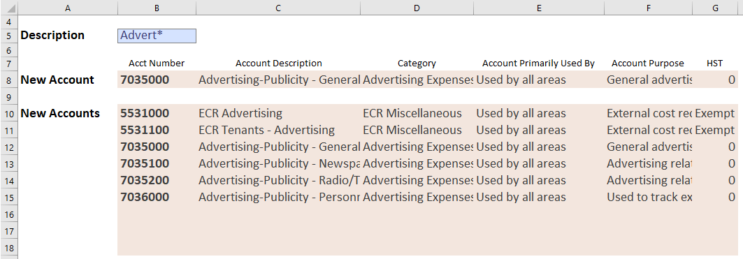
In the first result table in B8:G8, XLOOKUP is used to return multiple columns of data, rather than just the result from a single column. The third argument returns columns B to G, spilling right across the entire result table.
=XLOOKUP(B5,Accounts3[Account Description],Accounts3[[New Account]:[HST Status]],"",2,1)
However, what if there are multiple instances of ‘Advert*’ in the source table?
XLOOKUP can return the first instance, or the last instance by adjusting the sixth argument. But it does not (yet) support the ability to return an array with multiple hits. Hopefully that will be included in a future update to Excel.
Meanwhile, a formula using FILTER with a nested SEARCH provides equivalent results.
=FILTER(Accounts3[[New Account]:[HST Status]], ISNUMBER(SEARCH(B5,Accounts3[Account Description])))
SEARCH returns the starting position of one text string inside another, and supports wildcard searches. In this example, ISNUMBER determines whether SEARCH returns a numeric value or an error. In cases where SEARCH yields a number, that row is included in the FILTER result.
Summary
While HLOOKUP and VLOOKUP will likely be supported in Excel by Microsoft for years to come, there is probably no longer a use case for these that can not be handled better by XLOOKUP.
Download the XLOOKUP demo workbook.
Here are links to the Microsoft documentation for the XLOOKUP, IS and SEARCH functions.

Excel SEQUENCE Function
A final function to complete the dynamic array toolkit. Like some other DA functions, the function appears simple at first, but provides great versatility when combined with other DA functions such as UNIQUE, SORT and FILTER. For a discussion of dynamic arrays, see the intro to this series.
Usage
SEQUENCE provides the ability to create dynamic sequences of numbers or dates. This function is helpful with setting up amortization tables or forecasting models. It can even be used at the core of a dynamic calendar.
Arguments
The arguments are as follows.
| SEQUENCE(rows, [columns], [start], [step]) |
|---|
| rows = The number of rows to which the result should spill. |
| columns = The number of columns to which the result should spill. Default is 1. |
| start = Start number or date. Default is 1. |
| step = Amount by which the result should change. Default is 1. |
Examples
The examples below are available for download in the SEQUENCE demo workbook.
Example 1
To generate a column of 20 numbers starting at 10 and stepping by 10, the function would be as below.
=SEQUENCE(10,1,10,10)
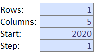
To set up a row of years, starting from 2020 for a 5-year forecasting model, use the following formula.
=SEQUENCE(1,5,2020,1)
In the demo workbook, use the SEQ_Numbers worksheet and adjust the amounts in the blue shaded cells to see how the results respond.
Example 2
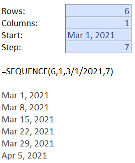
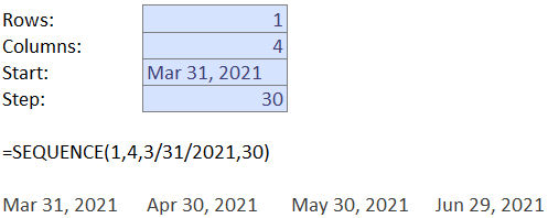
In the SEQ_Dates worksheet the function is similar, but results are formatted as dates.
With this example, one could generate a column of the next 6 Mondays, starting March 1, 2021, or column headings for an Accounts Receivable aging report.
Example 3
Until dynamic arrays were available in Excel, it was most common to provide scalar arguments to functions, that is, arguments that had a single value. However, now many Excel functions will accept arrays as arguments as well. This opens up many possibilities, especially for the SEQUENCE function.
(For those familiar with array or CSE or <Ctrl><Shift><Enter> formulas, that was and still is a way to work with array-based arguments and results. Though that capability is not dynamic in the way that the new DA functions are.)
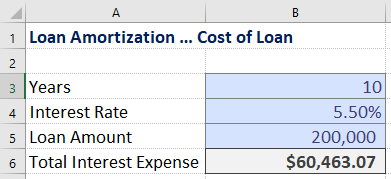
On the LoanCost worksheet of the demo workbook, the objective is to calculate total cost of a loan, provided with loan duration, interest rate and loan amount. This can be calculated in a single cell in B6.
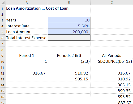
Start by reviewing the formula in cell A12. This uses the IPMT() function to calculate the interest portion of the loan payment for period 1.
=-IPMT(B4/12,1,B3*12,B5)
The second argument in the IMPT() function is the period for which to calculate interest. In cell B12, the 1 (scalar value) has been replaced with an array {2;3}. An array is formatted between curly brackets and separated by a semi-colon. This causes the result to spill, and return the interest portion of the loan payments for periods 2 and 3.
=-IPMT(B4/12,{2;3},B3*12,B5)
The formula in cell C12 then takes this to the next level by replacing the array {2;3} with a SEQUENCE() function containing all the values for the months in the loan, or B3 (loan duration in years) X 12.
=-IPMT(B4/12,SEQUENCE(B3*12),B3*12,B5)
Finally, to calculate total interest cost of the loan defined in cells B3 to B5, enclose the formula in cell C12 in a SUM().
=SUM(-IPMT(B4/12,SEQUENCE(B3*12),B3*12,B5))
Example 4
In the LoanAm worksheet, the SEQUENCE() function plays a key role in the construction of a dynamic loan amortization table.
Cells B3 to B5 contain the same inputs as the previous example. Cell B6 now uses the Excel PMT() function to calculate the monthly loan payment.
Cell D10 starts the amortization table with the initial loan amount.
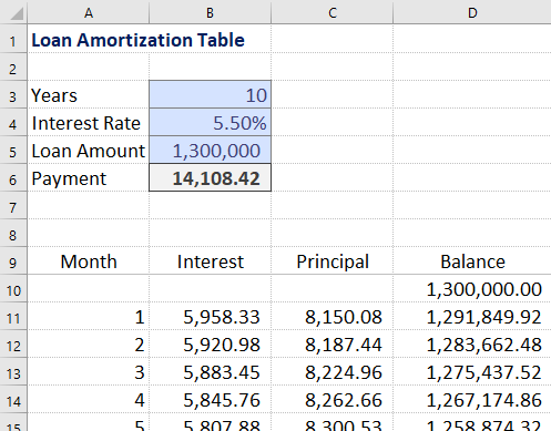
In row 11, the table calculations begin.
The Month column uses SEQUENCE() to return the month numbers, based on loan duration in years multiplied by 12.
The Interest column uses IPMT() function together with SEQUENCE to calculate monthly interest, as demonstrated in the previous example.
The Principal column subtracts the interest from the payment. To use the correct amount of interest for the month, the formula references B11#, or the array of values calculated in the Interest column.
Finally, the running Balance column uses a nested SUMIFS() function to reduce the loan balance by the total principal paid to date.
Next…
Bonus: The SEQUENCE demo workbook contains a Calendar worksheet which demonstrates a dynamic month calendar based on the use of SEQUENCE(), WEEKDAY() and IF().
While this wraps up the series of posts about functions released to specifically leverage the dynamic array capabilities in Excel, two additional posts will cover the versatile XLOOKUP() function and the new LET() function.
Download the SEQUENCE demo workbook.
Here is a link to the Microsoft documentation for the SEQUENCE function.

Excel UNIQUE Function
This continues a multi-part discussion of some new features introduced in Excel in 2019 and 2020. This describes the capabilities of the UNIQUE function, especially when used in combination with previously reviewed dynamic array functions SORT and FILTER. For a discussion of dynamic arrays, see the intro to this series.
Usage
This is the function for which many have been waiting for some time. UNIQUE returns a list of unique values from a longer list. This functionality can also be provided by using a pivot table, or sorting and grouping a list. But in both of those situations, the resulting list does not update automatically as the dynamic array returned by UNIQUE does.
Arguments
The arguments are as follows.
| UNIQUE(array, [by_col], [exactly_once]) |
|---|
| array = Columns included in the result. Can be entire or part of source data set. |
| by_col = If data is in rows instead of columns, use TRUE. Default is FALSE or 0. |
| exactly_once = TRUE returns values that occur only once in the data set. FALSE returns values that occur once or more. Default is FALSE. |
Examples
These examples are available for download in the demo workbook. Sample data is fictional but is set in the context of a post-secondary institution.
Example 1
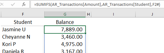
Starting with a raw list of financial transactions in a table called AR_Transactions that would be either linked to or exported from an accounting system, the objective is to compute current account balances.
Two formulas can be used to set this up. In F2, use the UNIQUE function to return a list of the names of students with transactions in the list. For readability, use the name of the table and column, rather than referring to the explicit cell range that includes the table and column.
=UNIQUE(AR_Transactions[Student])
In G2, use SUMIFS to simply add all the of transactions for each student.
=SUMIFS(AR_Transactions[Amount],AR_Transactions[Student],F2#)
The F2# refers to the entire dynamic array returned by UNIQUE into F2 and spilling down.
In the demo workbook for download, the SORT_UNIQUE worksheet has exactly the same data and table, but nests UNIQUE inside the SORT function to return a sorted list of student names.
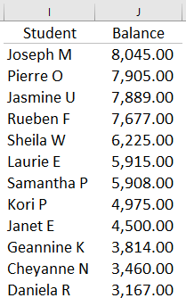
Of course, the most frequent question here is which student owes the most? A simple way to show this is to set up a dynamic array in cell I2 using this formula.
=SORT(F2#:G2#,2,-1)
This returns the spilled results in F2 and G2, sorts by the second column (the Balance), in descending order.
Example 2
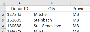
In this example, UNIQUE is used in combination with SORT to check for address errors or inconsistencies in a dataset of donor records.
The donor information is in a list in columns A to C. The data in this set is of course completely fictionalized, but the names of towns are from central Canada where Plains Edge is based.
Cells E2 and F2 contain the following formulas.
E2   =SORT(UNIQUE(B2:B301))

F2   =SORT(UNIQUE(C2:C301))
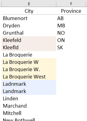
By sorting the unique results, many errors in the addresses are revealed. The village of Kleefeld is spelled two different ways, La Broquerie West is sometimes abbreviated in two different ways, and the name of Landmark is spelled incorrectly at least once.
Canadian provinces, like US states, can be abbreviated with two letters. AB and MB are correct abbreviations for Alberta and Manitoba. However, NO is not a valid identifier and is probably a transposition error for ON, or Ontario.
Application
In practice, the UNIQUE function is a tool that is often useful when evaluating a large dataset. How many customers are represented in the table? How many classifications are actually in use?
Used in combination, UNIQUE, SORT and FILTER functions can be used to create dynamic arrays in a wide variety of situations.
Download the UNIQUE demo workbook.
Here are links to the Microsoft documentation for the UNIQUE function.

Excel SORT Function
This is part of a multi-part discussion of some of the new features introduced in Excel in 2019 and 2020. This post is about one of the new dynamic array functions. For a discussion of dynamic arrays, see the intro to this series.
Usage
SORT does exactly what its name suggests. However, because it updates automatically, it is often a superior choice than a pivot table.
Arguments
The arguments are as follows.
| SORT(array, [sort_index], [sort_order], [by_col]) |
|---|
| array = Columns included in the result. Can be entire or part of source data set. |
| sort_index = The column index on which to sort. Default is 1. |
| sort_order = 1 for ascending, -1 for descending. Default is 1. |
| by_col = If data is in rows instead of columns, set to TRUE. Default is FALSE. |
Examples
These examples are all in the SORT demo workbook available for download. Note that data in the samples is fictional but is set in the context of a post-secondary institution.
Descending Order Sort
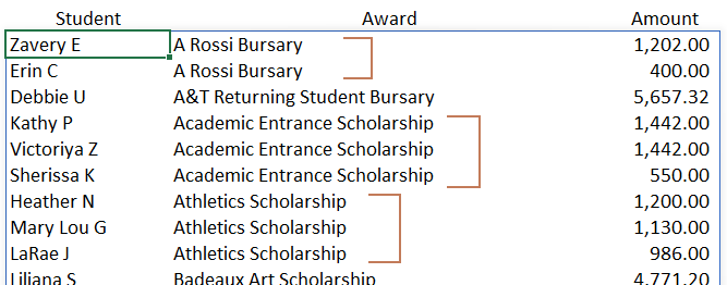
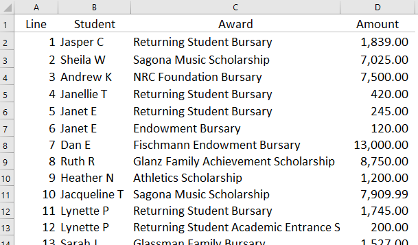
Using the list of student awards in range A2:D120, the following formula returns the set composed of student name, award name and amount (range B2:D120) sorted on the third column (the amount), in descending order.
=SORT(B2:D120,3,-1)
Multi-Column Sort
Using comma-separated arrays as arguments, it is fairly simply to define multiple sort columns and sort orders for each column.
To continue our example with student award data in A2:D120, we use SORT to retrieve 3 columns, the range B2:D120. Column 1 is the student name, column 2 the name of the award, and column 3 is the award amount. When we refer to index, we refer to the number of the column. To sort by column 2, then by column 3, we would put the 2 and then 3 inside curly brackets. {2,3}.
We’d also like to sort the awards in alphabetical ascending order, but continue to sort awards in descending order. For our sort_order argument, we then enclose a 1, then a -1, in curly brackets. {1,-1}.
Putting it all together, our SORT function is as follows:
=SORT(B2:D120,{2,3},{1,-1})
The SORTBY Function
When it is necessary to sort by a column that should not be included in the result, the SORTBY function can be used. The arguments for this function are as described below.
| SORTBY(array, [sort_array], [sort_order]) |
|---|
| array = Columns included in the result. Can be entire or part of source data set. |
| sort_array = The column on which to sort. |
| sort_order = 1 for ascending, -1 for descending. Default is 1. |
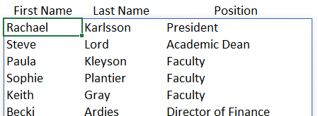
In the following example, staff names, positions and annual salaries are list in a table in A1:D16. This is formatted as a table (<ctrl><T>) named Staff. Using named tables with descriptive column names makes formulas much more readable.
The desired result is a list of names and positions, sorted in descending order by salary, without showing the salary. The SORTBY function identifies the array as Staff[[First Name]:[Position]], selecting the first three columns. The second argument identifies Staff[Salary] as the sort column. The final argument of -1 orders the result set in descending order.
=SORTBY(Staff[[First Name]:[Position]],Staff[Salary],-1)
In the final example, on sheet SORTBY2 of the demo workbook that can be downloaded here, the SORTBY and IF functions are used in a simple auditing tool to identify check numbers issued out of date sequence.
SINGLE
There are situations when the SORT or FILTER functions return an array, but a scalar, or single, result is required. In these situations, the function can be prefaced with the @ sign, or nested inside the SINGLE function.
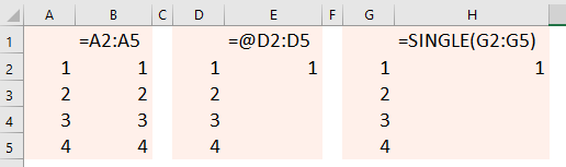
In the demo workbook on the SINGLE worksheet, the formula in B2 is =A2:A5. The result spills down from B2 to B5, as we have come to expect when working with array functions. However, in cell E2, the formula is =@D1:D5. In this case, the result is limited to a single value in E2. The same thing is accomplished with the =SINGLE(G2:G5) in cell H2.
Given a table named Employees in the range A1:D16, the SINGLE and SORTBY functions can be combined in a formula to return the name of the single highest-paid employee in the table.
=@SORTBY(Employees[Name],Employees[Salary],-1)
Looking Ahead
The SORT and SORTBY functions are deceptively simply. However, as we will begin to see in future posts, combining these with other functions unlocks some of their amazing potential.
Download the SORT demo workbook.
Here are links to the Microsoft documentation for the SORT, the SORTBY and the SINGLE functions.

Excel FILTER Function
This is part of a multi-part discussion of some of the new features introduced in Excel in 2019 and 2020. This post is about one of the new dynamic array functions. For a discussion of dynamic arrays, see the intro to this series.
Usage
FILTER is used to return a subset from a larger set of data based on specific criteria. It can even be used to return non-adjacent columns from the source set.
FILTER is a more flexible alternative to a pivot table, and can handle exceptions in a more robust manner than VLOOKUP.
Arguments
The arguments are as follows.
| FILTER(array, include, [if_empty]) |
|---|
| array = Columns included in the result. Can be entire or part of source data set. |
| include = Test to define what is included in result |
| if_empty = Result to return if filter returns no results. Default is at #CALC! error. |
Examples
These examples are all in the FILTER demo workbook available for download. Note that data in the samples is fictional but is set in the context of a post-secondary institution.
Simple Subset
In this first example, we are looking for a list of students who have received awards greater than $3,000 and the name of the award they received.
The entire list of awards is in the range B2:D120.
We type the following formula in cell F8:
=FILTER(B2:D120,D2:D120>3000,"None")
This returns only the columns we need with the student name, name of award, and amount of award where the amount of the award (in D2:D12) is greater than 3000. In the event that no awards exceed 3000, the formula would simply return the word “None”.

Of course, ‘>3000’ in the formula could be replaced with a reference to a specific cell, such as ‘>$G$5’ which could contain 3000 or any other value on which the return set should be filtered.
Multiple Filter Criteria
It is also possible to filter on more than one criteria. In this example, we would like to see awards with amounts between 3000 and 5000. This can be accomplished by placing the criteria in brackets and multiplying them.
=FILTER(B2:D120,(D2:D120>3000) * (D2:D120<5000),"None")
Multiplying the criteria combines these in a logical AND relationship. Adding the criteria would be the same as setting up OR criteria.
If we are looking for outlier points in our dataset of student awards, perhaps those with awards less than $200 or greater than $7,000, we would add the two criteria.
=FILTER(B2:D120,(D2:D120<200) + (D2:D120>7000),"None")
The result below then show only the small and the large awards, based on the criteria we specified.

Return Non-Adjacent Columns
By nesting one FILTER formula inside another, it is possible to return non-adjacent columns. In this final example, we would like to know which students received awards greater than $7,000, but we are not concerned with the type of award. Since the student name and award amount are not in adjacent columns, this poses a challenge since we can not specify multiple ranges in the first FILTER argument.
However, we can achieve our objective by nesting one FILTER formula inside another.
First we use FILTER to return columns B to D, filtering on the amount in column D.
Then we filter that result to return only the first and third columns, using an array of 1’s and 0’s to indicate which columns should be returned.
Note also that we have replace the third argument inside the inside FILTER function with an array of 3 values, {“None”,0,0}. Should there be no results greater than $7,000, our inside FILTER will return a result array with a width of 3 columns, suitable for the outside FILTER function to parse. Otherwise the outside FILTER function would return a #VALUE! error.
=FILTER(FILTER(B2:D120,D2:D120>7000,{"None",0,0}),{1,0,1})
Looking Ahead
This wraps up our quick introduction to the FILTER function. In future posts we’ll discover how combining FILTER with other new functions such as SORT and UNIQUE opens up intriguing new possibilities in Excel.
Download the FILTER demo workbook.
Here’s a link to the Microsoft documentation for the FILTER function.

Excel Re-Imagined
There are many sophisticated reporting and budgeting, forecasting and analysis tools on the market. Much of the marketing messaging around that software challenges us to ditch Excel in favor of their tool. They tell us Excel workbooks are prone to errors, don’t scale well, don’t handle succession well, and are subject to file corruption. It may all be true. But when everybody else has left for the day, we head back to our office and check those numbers in Excel.
In September 2018, Microsoft released seven new Excel functions to Office users subscribed to the Microsoft Insiders program. These are now generally available to Excel users. The new functions: UNIQUE, SORT, SORTBY, FILTER, RANDARRAY, SEQUENCE and SINGLE, can return multiple values, or dynamic arrays, to their own and neighboring cells. The result is a completely new set of Excel-based tools in the hands of business officers. In this new series of article we’ll look at these functions and how they trigger a whole new way of working inside Excel.
But first, we need to understand some changes to the Excel calculation engine.
Dynamic Arrays
Arrays: A set of elements that have some property in common.
In Excel, much of what we do involves working with an array. We are either processing the array in some way or analyzing it to discover useful information. Arrays can be either used as the output, or as a source for a lookup. Example: An array might be a list of US states or Canadian provinces with columns for their 2-letter identifier and their name. That array is pretty much static – there is no immediate expectation that it will add or lose members.
In Excel, a dynamic array is an array that can change. If the result of one of the new Excel functions returns a dynamic array that might not be limited to a single cell, that has to change the design of many spreadsheets.
To see if the version of Excel you are running supporting dynamic arrays, try this simple test.
Type a sequence of numbers in cells A1 through A4.
In cell B1, type ‘=A1:A4’ and press <Enter>
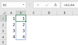
If your version of Excel supports dynamic arrays, the result of the short formula you typed in B1 will spill from from B1 to B4.
Spilling
Where we previously used array formulas (where we would press <Ctrl><Shift><Enter>), now it is sufficient to type in a formula and provide room on the sheet for the result to spill.
Or, if we previously typed one formula, then filled it down, we can now type a single formula, and the updated Excel calculation engine will spill the results. This works for the new Excel functions we’ll discuss in subsequent articles, but also previously existing functions.
In the example at the right, the ROUND() function spills when provided with a range as the first argument.
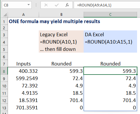
This behavior is exhibited both vertically and horizontally – a result spills down, or to the right.
Note the blue border around the results is a visual cue to the fact that the values in those cells are spilled formula results.
To delete spilled data, delete only the formula at the top of the column.
Cell formatting does not spill. However, formatting can be applied to the cells into which results spill.
In formulas that rely on the spilled data, a good way to reference the spilled result is to use the # sign. In the illustration of the ROUND() formula above, one could type a formula that refers to C8# that will then include the results from C8 to C13.
If there is data that interferes with the range to which data would spill, the formula returns a #SPILL error, and the range that must be cleared is outlined in a dashed blue border.
Over the next few articles, we’ll take a look at some of the new Excel functions that leverage the new capabilities of the redesigned Excel calculation engine.